Deployment Speed as a Cost Variable in SMB Technology Implementations
Faster deployment cuts the hidden cost of manual work that continues during implementation.
Deployment speed changes the cost and schedule of an SMB technology implementation. Every week a workflow stays manual adds labor spend, postpones useful capacity, and delays the next improvement a working system could support. The right comparison is therefore not just what each system costs to buy, but what it costs to wait for it to work.
Why deployment timeline is a cost variable, not a project management preference
SMBs often treat an implementation timeline as a logistics question, including when people are available, when training can happen, and when the project will finish. Yet that schedule is also doing something to the profit and loss statement. Until the replacement works in production, the business keeps paying for the process it plans to replace. The delay belongs in the financial comparison, even if it never appears on the vendor’s invoice.
A system that takes 12 weeks to deploy instead of 4 weeks brings in no return during those 8 extra weeks. The labor consumed in that interval cannot be recovered, and the capacity the system would have freed was not available. That makes a longer timeline a cost to weigh against any benefit from broader scope or a different delivery model.
What manual workflows actually cost while a replacement system is being built
The simplest place to measure that cost is the work already happening. In the accounting firm case, an office manager spent roughly 25–30 hours on client onboarding admin at a pace of 6–7 new clients per month. Those hours were a recurring demand on someone’s paid time. Using the office manager’s loaded compensation to price those hours shows the business how much the labor tied up in onboarding costs.
That calculation matters before and during the build. Even after an implementation agreement is signed, the next client still needs onboarding. The office manager still does the work while the replacement is being scoped, built, and connected. If the implementation takes longer, the business pays for more of those hours before the system starts saving time. Treating them only as a description of the old process leaves part of the deployment cost out of the comparison.
The cost of waiting also applies to work done by an operations coordinator, whose fully loaded annual cost is tens of thousands of dollars. An automation does not have to replace that person for the time it releases to matter. However, released hours and reduced payroll are not the same thing, so the calculation should distinguish labor capacity from cash savings. SMBs have less slack to absorb manual work than larger organizations, making that capacity a larger share of the operating budget. Most budget for the new system, but few put a figure on the period before they have it.
How the choice of delivery model sets the deployment clock before a line of code is written
The choice among an internal hire, a SaaS tool, DIY automation, and an agency engagement is usually presented as a comparison of features and price. It is also a choice about how the work reaches production. Each model gives someone different the responsibility for building and connecting the system. That responsibility determines how much must happen before the business gets a working replacement.
With an internal build, people inside the business develop the system and hold its institutional knowledge. But if the engineer leaves before it ships, that knowledge leaves too, and the clock can reset. DIY automation platforms suit simple, stable processes, but they reach a ceiling when the work needs AI reasoning, cross-tool context, or recurring intelligence outputs. In that situation, a quick build may leave the actual bottleneck untouched. A SaaS tool also has to be judged by whether it replaces the workflow.
An agency or embedded engagement can compress the timeline because an experienced team scopes, builds, and integrates in parallel. Delivery models differ in how they structure the work. If one delivery model takes six months longer, the business pays for six months of manual work as well as the implementation bill. That difference can change which option is cheaper without changing either quoted price.
The 30-day threshold and what it separates
A 30-day first deployment gives that comparison a practical benchmark. It tests whether the proposal can produce useful work soon or needs a long sequence of prerequisites before anything changes. The pattern in the documented deployments favors a single, high-frequency, repetitive workflow, such as document processing, scheduling, FAQ response, or data entry. These tasks give the first system a clear job to do again and again, with output that can be measured. The threshold is a diagnostic tool, with payback within a month remaining uncertain even for suitable projects.
The HVAC company case shows what a tightly defined workflow can deliver. Its implementation combined AI call answering, automated scheduling, and follow-up sequences at a modest monthly cost. Call answer rate and booking conversion rose by a lot, while admin time dropped by 20 hours per week. The payback period was 31 days, approximately one month. That result depended on getting the connected workflow into use quickly, rather than spending the early period on a broad pilot.
The accounting firm’s onboarding workload illustrates another part of the same test. The steady flow of new clients and the many hours spent on admin showed how much work the firm had at the start, giving it a baseline for measuring how much an implementation helped. The shared characteristics are frequency, a consistent pattern, and enough current time consumption for a change to register. By contrast, a multi-department project that tries to solve everything at once has more to complete before returns begin. The 30-day frame exposes that difference without pretending the accounting case establishes the same payback period as the HVAC case.
Why most AI pilots stall before they pay back, and what that failure mode reveals
The strongest objection is that most AI pilots stall before paying back, so a shorter build alone cannot establish value. That objection is valid. A fast demonstration is still a demonstration if it does not change the work people do. Pilots disconnected from the CRM, ERP, or actual operating workflow may generate data without producing useful operational output. Their payback clock never starts, regardless of how quickly the demonstration was assembled.
This failure mode narrows what deployment must mean. It has to mean that the system is connected to a real workflow and doing useful work. Speed and integration are therefore joint requirements.
Vendor-partnered deployments succeed at roughly twice the rate of internal builds, which suggests that how the work is delivered matters beyond who is hired to do it. It does not make any particular engagement certain to succeed. Rather, it is consistent with the value of focused delivery that reaches the workflow instead of stopping at demo polish. The test is whether the proposed first system can generate measurable output from recurring work within 30 days.
Hidden costs still matter, including data preparation, integration complexity, change management, and ongoing maintenance. These can push total costs above the initial estimate even when the underlying technology works. The response is to scope the first deployment narrowly enough to absorb those costs and still pay back quickly. Narrow scope means limiting the first job so that the necessary integration remains a bounded project.
How value compounds once a working system is live, and why that makes early deployment disproportionately valuable
Once the system does useful work, the benefit can extend beyond the hours saved on its first task. Freed capacity lets the team take on higher-value work. That work can generate revenue or retention gains, which can fund or justify the next deployment. It can also reveal the next bottleneck more clearly. The return compounds through expanded capability.
For a five-person team, that distinction is important. The constraint may be the number of hours available. A working system removes part of that operational ceiling in the area it covers. The business can then do more in that area without adding headcount. This is a different goal from using automation only to shrink the cost of an unchanged workload.
SANSA’s model follows this path by diagnosing the highest-leverage bottleneck in two weeks, deploying a production-ready system around it, and staying embedded as it compounds. In its insurance broker example, manual data entry fell by 80%, while its freight company example saved 160+ hours per month. These results establish the first release of capacity that the compounding model depends on. They do not, by themselves, quantify every later revenue or retention gain. Their significance is that less of the team’s time is locked into the original bottleneck.
That is why a system deployed in week 4 rather than week 16 offers more than a 12-week head start on repayment. It also gives the business 12 more weeks in which released capacity can support the next capability. That next step depends on replacing the first manual workflow. Delay postpones both the initial improvement and the chance to build on it. Early deployment is disproportionately valuable because it starts the sequence of savings and expanded capability.
How to evaluate a proposed AI implementation using deployment timeline as a cost variable
Start a proposal review by asking when the first workflow will be live and producing measurable output. Separate that date from the dates for a demo, tool access, or the completion of a planning phase. Then calculate the manual labor cost expected to accumulate until production begins, using the workflow’s current hours and loaded compensation. Keep the value of the time freed up separate from any drop in what the business spends. This gives the timeline a financial weight that can be compared with price, scope, and features.
Next, ask whether the first deployment covers a single workflow that happens frequently, follows a consistent pattern, and consumes significant team time. If it does not meet all three conditions, take a closer look at the proposed payback. Ask what integration, data preparation, and change management must be done before the system can start doing the work. See whether the first scope is small enough to meet those needs promptly. A narrow first deployment makes it easier to contain hidden costs without leaving the workflow disconnected.
Then ask who owns the path from diagnosis to production and what happens after launch. An embedded engagement, where a specialist builds inside the existing stack and stays to iterate, is one option that fits this framework. SANSA offers SMBs one example of this: a two-week diagnostic followed by a production-ready build. Judge that structure by whether scoping, building, and integration can happen at the same time, rather than taking the engagement’s name as a promise of speed. Include maintenance in the budget so that the comparison extends beyond getting the first system live.
Finally, compare the proposals using the cost of waiting as well as the cost of buying. A lower quote can lose its advantage if the business must carry the manual workflow for much longer. For a faster proposal to be worth the head start, the system has to connect to the workflow and do the work. Evaluating an AI implementation without calculating the cost of its deployment timeline is like evaluating a loan without calculating the interest. The sticker price is not the total cost, and deployment speed can change which option is actually cheaper.